P&S Module 2019

Welcome to the first session of the module — Deep Learning on Raspberry Pi.

In this session, we will revisit the basic concepts of Linear Algebra. Then, we will familiarize ourselves with numpy, a Python package used for scientific computing and some basics of symbolic computation. At the end of this session, there will be a few exercises which will further help to understand the concepts introduced here.

Linear Algebra

This section will only provide a brief introduction to Linear Algebra. For those of you who are unfamiliar with the concepts of Linear Algebra, it is strongly recommended that you spend some time with a text book or complete a course on Linear Algebra. A strongly recommended text book is Introduction to Linear Algebra by Gilbert Strang.

Remarks: In this module, we do not emphasize the geometry aspects of the Linear Algebra. Instead, we use the relevant concepts for programing and computation.

Scalar, Vector, Matrix and Tensor

A Scalar is just a single number.
A Vector is an array of numbers. These numbers are arranged in order. For example a vector $\mathbf{x}$ that has $n$ elements is represented as:

A numpy example of a 6-element vector is given as follows:
```
  np.array([1, 2, 3, 4, 5, 6])  # a row vector that has 6 elements
```
Remarks: by default, numpy can only represent row vector because numpy needs two dimensions to represent a column vector.
A Matrix is a 2D array of numbers. Matrices are mainly used as linear operators to transform a vector space $\mathbb{R}^m$ to $\mathbb{R}^n$ , which would be an $n\times m$ matrix represented as:

A numpy example:
```
  np.array([[1, 2, 3, 4],
            [5, 6, 7, 8],
            [9, 10, 11, 12]])  # a 3x4 matrix
```
The matrix transpose is defined as $\mathbf{A}^{\top}$ where $(\mathbf{A}^{\top}_{i,j})=\mathbf{A}_{j,i}$ . The transpose of the matrix can be thought of as a mirror image across the main diagonal. Python has a nice API for the matrix:
```
  A_transpose = A.T
```
A multi-dimensional array is called a tensor. Note that scalars are 0-dimensional tensors, vectors are 1-dimensional tensors and matrices are 2-dimensional tensors.
```
  np.ones(shape=(2, 3, 4, 5))  # a 4D tensor that has 2x3x4x5 elements which are filled as 1
```

Matrix Arithmetic

Add between matrices
$\mathbf{C}=\mathbf{A}+\mathbf{B}\quad\text{where }\mathbf{C}_{i,j}=\mathbf{A}_{i,j}+\mathbf{B}_{i,j}$
Add or multiply a scalar
$\mathbf{D}=a\cdot\mathbf{B}+c\quad\text{where }\mathbf{D}_{i,j}=a\cdot \mathbf{B}_{i,j}+c$
Matrix multiplication, the product of two matrices $\mathbf{A}\in\mathbb{R}^{m\times n}$ and $\mathbf{B}\in\mathbb{R}^{n\times p}$ is the matrix $\mathbf{C}$ :
$\mathbf{C}=\mathbf{A}\mathbf{B}$
where
$\mathbf{C}_{i,j}=\sum_{k=1}^{n}\mathbf{A}_{i,k}\mathbf{B}_{k,j}$
Note that matrix multiplication is order dependent, which means $\mathbf{A}\mathbf{B}\neq\mathbf{B}\mathbf{A}$ (not always). There are many useful properties. For example, matrix multiplication is both distributive and associative:
$\mathbf{A}(\mathbf{B}+\mathbf{C})=\mathbf{A}\mathbf{B}+\mathbf{A}\mathbf{C}$ $\mathbf{A}(\mathbf{B}\mathbf{C})=(\mathbf{A}\mathbf{B})\mathbf{C}$
The transpose of a matrix product is:
$(\mathbf{A}\mathbf{B})^{\top}=\mathbf{B}^{\top}\mathbf{A}^{\top}$

Identity and Inverse Matrix

The identity matrix $\mathbf{I}\in\mathbb{R}^{n\times n}$ is a special square matrix where all the entries along the diagonal are 1, while all other entries are zero:

$\mathbf{I}_{i,i} = 1, \mathbf{I}_{i,j_{i\neq j}}=0$

The identity matrix has the nice property that it does not change a matrix that it is multiplied with:

$\mathbf{I}\mathbf{A}=\mathbf{A}$

The matrix inverse of $\mathbf{A}$ is denoted as $\mathbf{A}^{-1}$ , and it is defined as the matrix such that:

$\mathbf{A}\mathbf{A}^{-1}=\mathbf{I}$

Remarks: Not all matrices have a corresponding inverse matrix.

Norms

We use the concept of norm to measure the size of a vector. Formally an $L^{p}$ norm of a vector $\mathbf{x}$ is given by:

$||\mathbf{x}||_{p}=\left(\sum_{i}|x_{i}|^{p}\right)^{\frac{1}{p}}$

for $p\in\mathbb{R}$ , $p\geq 1$ .

The most common norms are $L^{1}$ , $L^{2}$ and $L^{\infty}$ norms:

$\begin{aligned} L^{1}:& \|\mathbf{x}\|_{1}=\sum_{i}|\mathbf{x}_{i}| \\ L^{2}:& \|\mathbf{x}\|_{2}=\sqrt{\sum_{i}\mathbf{x}_{i}^{2}} \\ L^{\infty}:& \|\mathbf{x}\|_{\infty} = \max_{i}|\mathbf{x}_{i}| \end{aligned}$

Trace Operator

The trace operator gives the sum of all the diagonal entries of a matrix:

$\text{Tr}(\mathbf{A})=\sum_{i}\mathbf{A}_{i,i}$

There are many useful yet not obvious properties given by the trace operator. For example, for $\mathbf{A}\in\mathbb{R}^{m\times n}$ and $\mathbf{B}\in\mathbb{R}^{n\times m}$ , we have:

$\text{Tr}(\mathbf{A}\mathbf{B})=\text{Tr}(\mathbf{B}\mathbf{A})$

even though $\mathbf{A}\mathbf{B}\in\mathbb{R}^{m\times m}$ and $\mathbf{B}\mathbf{A}\in\mathbb{R}^{n\times n}$ .

Remarks: We do not intend to present a full review of Linear Algebra. For those who need to quickly learn the material, please read Chapter 2 of the Deep Learning Book or Linear Algebra Review and Reference. Both resources give a very good presentation on the topic.

Basic numpy

The contents of this section are mainly based on the quickstart tutorial of numpy from the official website.

The main object in numpy is the homogeneous multi-dimensional array (or a tensor). The main difference between a Python multi-dimensional list and the numpy array is that elements of a list can be of different types, while the elements of a numpy array are of the same type.

numpy’s array class is called the ndarray, which also goes by the alias array. A few important attributes of the ndarray object are ndarray.shape which has the dimensions of the array, ndarray.dtype which has the type of elements in the array (e.g., numpy.int16, numpy.float16, numpy.float32, etc).

Let us look at an example.

# this statement imports numpy with the alias np
# which is easier to use than the whole word 'numpy'
import numpy as np

# creates an array (0, 1, 2, ..., 14)
a = np.arange(15)

# should output (15,)
a.shape

# reshapes the above array of shape (15,) into (3, 5)
# notice the number of elements is still the same
a = a.reshape(3, 5)

# should output (3, 5)
a.shape

# type of the elements in the array
# should output int64, since it is the default dtype for the function arange
a.dtype

# recasts the elements of a into type int8
a = a.astype(np.int8)

# should output int8
a.dtype

To operate on numpy arrays, they have to be created. numpy arrays can be created in many ways.

# initialize from a list with the dtype float32, the dtype unless specified is int64 since
# the numbers in the list are integers
np.array([[1, 2], [3, 4]], dtype=np.float32)

# created an array initialized with zeros, the default dtype is float64
np.zeros(shape=(2, 3))

# fill an array with ones
np.ones(shape=(2, 3))

# linspace like the matlab function
np.linspace(0, 15, 30)  # 30 numbers from 0 to 15

Now that the arrays are created, let us look at how the arrays can be operated on. The arithmetic operations on arrays are applied element wise.

a = np.array([[1, 2], [3, 4]], dtype=np.float32)
b = np.array([[1, 1], [2, 2]], dtype=np.float32)
# subtracting one array from another element wise
a - b

# adding two arrays element wise
a + b

# multiplying two arrays element wise
a * b

# squaring the elements of each array
a ** 2

# applying the sine function on the array multiplied with pi / 2
np.sin(a * np.pi / 2)

# for the matrix product, there is a dot function
np.dot(a, b)

# element wise exponential of the array subtracted by 2
np.exp(a - 2)

# square root of the array element wise
np.sqrt(a)

Arrays of different types can be operated, the resulting array corresponds to the dtype of the more general or the more precise one.

a = np.array([[1, 2], [3, 4]], dtype=np.float64)
b = np.array([[1, 1], [2, 2]], dtype=np.float32)

c = a + b

# should be of type float 64
c.dtype

a = a.astype(np.int64)
c = a + b

# should be of type float 64
c.dtype

numpy also provides inplace operations to modify existing arrays.

a = np.array([[1, 2], [3, 4]], dtype=np.float32)
b = np.array([[1, 1], [2, 2]], dtype=np.int32)

# adds the matrix b to the matrix a
a += b

# note that when trying to add a to b you get an error
b += a

There are many inbuilt unary operations as well, the names are self explanatory.

a = np.array([[1, 2, 3], [4, 5, 6]])

# sum of all elements in the array
a.sum()

# sum of all elements along a particular axis
a.sum(axis=0)

# minimum of all elements in the array
a.min()

# -1 corresponds to the last dimension, -2 for the last but one and so on
# computes the cumulative sum along the last axis
a.cumsum(axis=-1)  

While 1D arrays can be indexed just like python native lists, multi-dimensional arrays can have one index per axis. These indices are in an n-length tuple for an n-dimensional array.

a = np.arange(12)

a[2:5]  # indexes the 2nd element to the 4th element
# notice that the last element is the 4th element and not the 5th

# From the fifth element, indexing every two elements
a[4::2]

a = a.reshape(3, 2, 2)

a[:, 1, :]  # a simple colon represents all the elements in that dimension

# 1: indexes the 1st element to the last element whole
# :-1 indexes the 0th element to the last but one element
a[1:, :, 0]

Iterating over multidimensional arrays is done with respect to the first axis.

a = np.arange(12).reshape(3, 2, 2)

for element in a:
  print(element)

for element in np.transpose(a, axes=[1, 0, 2]):
  print(element)

numpy broadcasts arrays of different shapes during arithmetic operations. Broadcasting allows functions to deal with inputs that do not have the same shape but expect inputs that have the same shape.

The first rule of broadcasting is that if all the input arrays do not have the same dimensions, a ‘1’ will be prepended to the shapes of the smaller arrays until all the arrays have the same number of dimensions.

The second rule ensures that arrays with size ‘1’ along a particular dimension act as if they had the size of the largest array in that dimension, with the value repeated in that dimension.

After these two rules, the arrays must be of the same shape, otherwise the arrays are not broadcastable. Further details can be found here.

a = np.arange(4)
b = np.arange(5)

a + b  # throws an exception

c = a.reshape(4, 1) + b

c.shape

Remarks: Some of you might realize that we use numpy to manipulate array instead of matrix. And in fact, there is a data structure in numpy that is dedicated to matrix manipulation. However, matrix is a derived type of array and less flexible. Therefore, in this module and practice, we always use ndarray.

Remarks: For a more complete Python numpy Tutorial, please check this document from Stanford CS231n class.

Basic Symbolic Computation

While classical computing (numerical computing) defines variables and uses operations to modify their values, symbolic computation defines a graph of operations on symbols, which can be substituted for values later. These operations can include addition, subtraction, multiplication, matrix multiplication, differentiation, exponentiation, etc.

Every operation takes as input symbols (tensors), and outputs symbols that can be further operated upon.

In this module, we will use TensorFlow, a dedicated machine learning framework based on symbolic computation. Specifically, we use the official high-level API – Keras.

Remarks: Keras is an open source project that was dedicated to providing a clean yet efficient high-level API that unifies several different frameworks. Keras has become the official high-level abstraction layer of TensorFlow and has been deeply fused into recent TensorFlow releases. Therefore, for this module, we choose to use Keras in TensorFlow to get better support and performance.

Remarks: Almost all modern Deep Learning libraries follows the principles of symbolic computation including Theano, TensorFlow, PyTorch, MXNET, Chainer, etc.

First let us import the backend functions of Keras in python and implement some basic operations.

import numpy as np
from tensorflow.keras import backend as K

Now initialize two input scalars (shape () tensors) which can then be added together. Placeholders are basic tensor variables which can later be substituted with numpy arrays during the evaluation of the further operations.

input_1 = K.placeholder(shape=())
input_2 = K.placeholder(shape=())

print(input_1)

inputs_added = input_1 + input_2

print(inputs_added)

Now we can instantiate an add function from the symbols created above.

add_function = K.function(inputs=[input_1, input_2],
                          outputs=[inputs_added])
print(add_function)

This add function takes on two scalars as inputs and returns a scalar as an output.

add_function((37, 42))

Similarly, you can also add two matrices of the same shape instead of scalars.

input_1 = K.placeholder(shape=(2, 2))
input_2 = K.placeholder(shape=(2, 2))

inputs_added = input_1 + input_2

add_function = K.function(inputs=[input_1, input_2],
                          outputs=[inputs_added])

add_function((np.array([[1, 3], [2, 4]]),
              np.array([[3, 2], [5, 6]])))

The above code represents a computation graph which takes two inputs and gives one output (see a graphical example below).

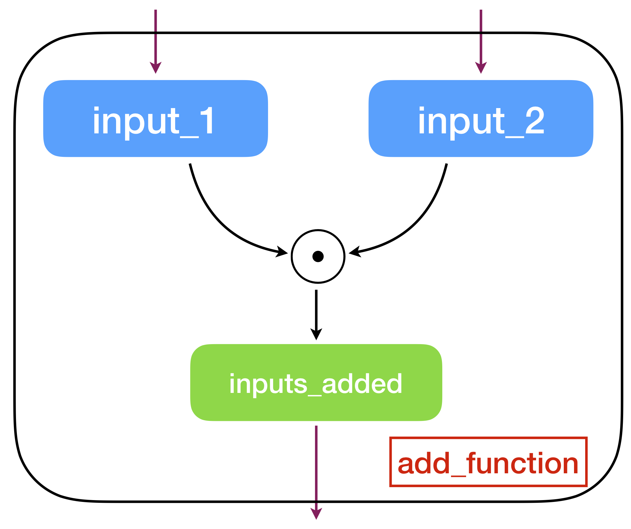
An example of a computation graph.

Computation graph is the essential concept of symbolic computation where the tensors in this case define the steps of the computation and the graph compilation (achieved by K.function API) turns the graph into a function. Note that before compiling, the elements in the graph are merely symbols. The main advantage of using symbolic computation is automatic differentiation which can be directly derived from a graph. Almost all training algorithms in deep learning rely on this powerful technique.

For this, we need to get acquainted with keras variables. While keras placeholders are a way to instantiate tensors, they are placeholder tensors for users to substitute values into to carry out their intended computation. Variables are tensors that have initial values.

# we redefine the input_1 and input_2 tensors
input_1 = K.placeholder(shape=(2, 2))
input_2 = K.placeholder(shape=(2, 2))

# variable can be initialized with a value like this
init_variable_1 = np.zeros(shape=(2, 2))
variable_1 = K.variable(value=init_variable_1)

# variable can also be initialized with particular functions like this
variable_2 = K.ones(shape=(2, 2))

add_tensor = input_1*variable_1+input_2*variable_2

print("Variable 1:", variable_1)  # note that it doesn't print the value contained
print("Added tensors together:", add_tensor)

# notice the difference in the types, one is a variable tensor
# while the other is just a tensor

# we can evaluate the value of variables like this
print("Values in variable 1:", K.eval(variable_1))
print("Values in variable 2:", K.eval(variable_2))

# we can create the add function from the add_tensor just like before

add_function = K.function(inputs=[input_1, input_2],
                          outputs=[add_tensor])

print(add_function((np.array([[1, 3], [2, 4]]),
                    np.array([[3, 2], [5, 6]]))))
# notice that the add_function created is independent of the variables
# the value of variables created is not affected

print("Variable 1:", K.eval(variable_1))
print("Variable 2:", K.eval(variable_2))

# we can set the value of variables like this
K.set_value(x=variable_1, value=np.array([[1, 3], [2, 4]]))

print("Variable 1 after change:", K.eval(variable_1))

# notice that the change in variable_1 is reflected when you call add_function again

print(add_function((np.array([[1, 3], [2, 4]]),
                    np.array([[3, 2], [5, 6]]))))

Remarks: As defined in the function API, the input tensors have to be a list of placeholders. TensorFlow’s Keras strictly follows this definition. However, the original Keras does not care if the input tensors are placeholders or variables. This is a bug of current TensorFlow since function could run without warning when variables are passed as input. See here.

We can also compute more than one thing at the same time by using multiple outputs. Say we want to add two tensors, subtract two tensors, perform an element-wise squaring operation on one of the tensors and get the element-wise exponential of the other tensor.

# we redefine the input_1 and input_2 tensors
input_1 = K.placeholder(shape=(2, 2))
input_2 = K.placeholder(shape=(2, 2))

add_tensor = input_1 + input_2
subtract_tensor = input_1 - input_2
square_1_tensor = input_1 ** 2
exp_2_tensor = K.exp(input_2)

multiple_output_function = K.function(inputs=(input_1, input_2),
                                      outputs=[add_tensor,
                                               subtract_tensor,
                                               square_1_tensor,
                                               exp_2_tensor])

multiple_output_function((np.array([[1, 3], [2, 4]]),
                          np.array([[3, 2], [5, 6]])))

Now we can get to the important part of differentiating with respect to the variables. Once we have created the variables and performed operations of interest on them, we would like to get the gradients of the output symbols from those operations with respect to the variables.

# we redefine the input_1 and input_2 tensors
input_1 = K.placeholder(shape=(2, 2))
input_2 = K.placeholder(shape=(2, 2))

variable_1 = K.ones(shape=(2, 2))
variable_2 = K.ones(shape=(2, 2))


square_1_tensor = input_1*variable_1**2+input_2*variable_2**2
exp_tensors_added = K.exp(input_1*variable_1) + K.exp(input_2*variable_2)

# we can compute the gradients with respect to a single variable or
# a list of variables

# computing the gradient of square_1_tensor with respect to variable_1
grad_1_tensor = K.gradients(loss=square_1_tensor, variables=[variable_1])

# computing the gradient of square_1_tensor with respect to variable_2
grad_2_tensor = K.gradients(loss=square_1_tensor, variables=[variable_2])

# computing the gradient of exp_tensors_added with respect to both
# variable_1 and variable_2
grad_3_tensor = K.gradients(loss=exp_tensors_added,
                            variables=[variable_1,
                                       variable_2])

# we can now create functions corresponding to these operations
grad_functions = K.function(inputs=[input_1, input_2],
                            outputs=[grad_1_tensor[0],
                                     grad_3_tensor[0],
                                     grad_3_tensor[1]])

grad_functions((np.array([[1, 3], [2, 4]]),
                np.array([[3, 2], [5, 6]])))

Remarks: The complete API reference is available at Keras documentation for backend.

In this session, we learned basic ideas in symbolic computation. Some of you may have heard that another popular library PyTorch is even easier to use than TensorFlow. PyTorch uses a framework called dynamic computation graph which can generate the graph on the fly. This means that it is closer to our old programming paradigm. However, to think the computing differently, in this module we keep using the static computation graph.

Exercises

Create three symbolic placeholder vectors of length 5 (shape (5,) tensors) $\mathbf{a}$ , $\mathbf{b}$ and $\mathbf{c}$ ; then create a function to compute the expression $\mathbf{a}^2 + \mathbf{b}^2 + \mathbf{c}^2 + 2\mathbf{b}\mathbf{c}$ . (Element-wise multiplication)
Create a scalar placeholder $x$ and compute the $\tanh$ function on $x$ using the exponential function (DO NOT USE K.tanh API). Then compute the derivative of the $\tanh$ with respect to $x$ using the gradients function. Invoke the functions with the values -100, -1, 0, 1 and 100 to analyze the function and its derivative.
Create shape (2,) variable $\mathbf{w}$ and the shape (1,) variable $\mathbf{b}$ . Create shape (2,) placeholder $\mathbf{x}$ . Now create the function corresponding to $f(z) = \frac{1}{1+e^{-z}}$ where $z=w_0\times x_0+w_1\times x_1+b_0$ and compute the gradient with respect to $\mathbf{w}$ . Analyse the implemented operation. Then see how the function and the gradient behave for different values of the variables and the placeholder.
For an arbitrary $n$ , create an $n$ -degree polynomial for an input scalar variable $\mathbf{x}$ with $(n+1)$ variables and compute the gradients of the polynomial with respect to each of the variables.